Instrumental Variables
In this third post, I want to go into the details of a method mentioned in my previous post about Structural Causal Modeling called Instrumental Variables (IV). IVs have traditionally been used to estimate structural econometric models, but during the last decade, advocates have encouraged the broader use of IVs within social sciences (Bollen, 2012; Sovey & Green, 2011). One of its interesting characteristics is that IVs allow researchers to estimate causal relationships when randomized experiments are not feasible, so we need to use observational data.
Instrument
We can observe the setup of an IV \( (I) \) in Figure 1. As researchers, let’s say that we are interested in calculating the causal effect of \( X \) on \( Y \) \( (X \rightarrow Y) \). From our understanding of causal models, to know the correct causal effect of \( X \rightarrow Y \), we need to control for the confounders (in this case represented by the set of variables \( U \)) because if we don’t, there will be confounder bias in our estimation. But what can we do if the set of variables \( U \) is unobserved? Well, IVs allow us to estimate the causal effect of \( X \) on \( Y \) without measuring the set of confounders \( U \) as long as we can define the instrument variable \( I \). The variable \( I \) is an instrument if:
- \( I \) defines a causal relationship with \( X \).
- \( I \) affects to the outcome variable \( Y \) only through its effect on \( X \) (exclusion restriction).
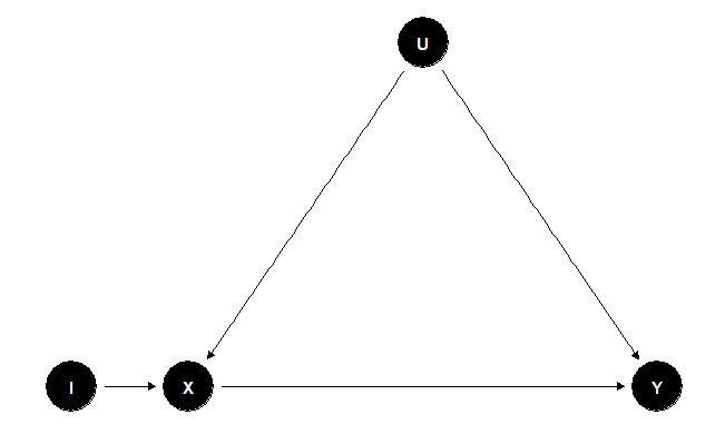
Figure 1
To illustrate a practical example of using IVs, let’s look at the work done by Coviello et al. (2014). In this paper, the authors studied the process of emotional contagion in a massive social network site; they wanted to know if the online emotional expression of users on Facebook affects the emotions their friends share on the same platform. To simplify the example with a particular case and following the setup of Figure 1, the variable \( X \) is defined as the average emotional expression of Yvonne’s friends’ status on Facebook, and variable \( Y \) is the emotional expression of Yvonne. Both \( X \) and \( Y \) are measured in the same period. For the instrument \( I \), a variable is needed that (1) defines a causal relationship with the emotional expression of Yvonne’s friends and (2) follows the exclusion restriction (affects Yvonne’s emotional expression through the emotions of her friends). The researchers picked rainfall as instrument \( I \); their justification was that if there is a relationship between rainfall and emotion expression, it must be \( rainfall \rightarrow emotion \) because emotions can’t affect rainfall; this rationale complies with (1). For the exclusion restriction (2), they computed the model when there was no rainfall in Yvonne’s city, so the instrument had no relationship with her emotional expression. The final general result showed that rainfall directly influences the emotional content status messages of users on Facebook, and it also affects the status messages of friends in cities that are not experiencing rainfall.
Analysis
The analysis of causal effects using IVs uses the additive properties of SEM to calculate the causal effect when we can define an instrument.
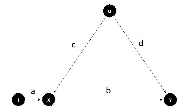
Figure 2
We already know that Figure 2 represents a setup for IVs. Here, we are interested in the causal effect of \( X \) on \( Y \). The variable \( I \) is a well-defined instrument, the set \( U \) represents the group of unobserved confounding variables, and a, b, c, and d the causal effects of the DAG assuming linear equations (if you need to refresh concepts like confounders or DAG take a look at my previous post).
Because \( I \) and \( X \) are unconfouded the causal effect of \( I \) on \( X \) can be estimated from the regression
\[ X = a I + error_1 \tag{1} \]
Likewise, the variables \( I \) and \( Y \) are unconfounded because the path \( I \rightarrow X \leftarrow U \rightarrow Y \) is blocked in the collider \( X \). So the estimate of the regression of \( I \) on \( Y \) will be equal to the direct effect on the path \( I \rightarrow X \rightarrow Y \), which is the product of the path coefficients \( ab \).
Since we estimated the values \( a \) and \( ab \). The causal effect \( b \) from \( X \) to \( Y \) can be obtained by dividing the previous estimations \( b=ab/a \) (Pearl & Mackenzie, 2018)
Limitations
Even though using IV might seem a good approach to fixing problems as confounding issues, the truth is that instruments can be very difficult to find. Researchers cannot use the actual data to find IVs; the knowledge about theory and the model derived from it is key to defining a valid IV for the problem under investigation. A well-defined IV should not be affected by other variables in the model; this can’t be proved, so it is based on the knowledge of the system studied. The correlation between the IV and \( X \) must be significant because weak correlations can lead to misleading parameter estimates and standard errors.
An Instrumental Variable Example
I present an example of Instrumental Variables with simulated data to show how to implement the previous analysis. The process has the following steps:
- Plot the IV model.
- Data simulation of the DAG defined.
- Check correlation between instrument \( I \) and variable \( X \).
- Estimate the causal effect of the IV model.
- Show the estimation mistakes if we don’t use IV for this example.
References
Bollen, K. A. (2012). Instrumental Variables in Sociology and the Social Sciences. Annual Review of Sociology, 38(1), 37–72. https://doi.org/10.1146/annurev-soc-081309-150141
Coviello, L., Sohn, Y., Kramer, A. D., Marlow, C., Franceschetti, M., Christakis, N. A., & Fowler, J. H. (2014). Detecting emotional contagion in massive social networks. PloS One, 9(3), e90315. https://doi.org/10.1371/journal.pone.0090315
Pearl, J., & Mackenzie, D. (2018). The Book of Why: The New Science of Cause and Effect. Basic Books.
Sovey, A. J., & Green, D. P. (2011). Instrumental Variables Estimation in Political Science: A Readers’ Guide. American Journal of Political Science, 55(1), 188–200. https://doi.org/10.1111/j.1540-5907.2010.00477.x